Every policy mining pipeline keeps its working under the heading How this was found: what it considered, what it kept and why, how each attribute was divided into bins, whether those bins remained stable over time, and the sweep behind the cutoff. This is the material a validator reads, and the part you can challenge before proposing anything.
- Attributes considered
- Derived quantities tried
- Binning and stability
- Three checks, and the worst one wins
- Reading the stability panel
- Scorecard bins with WOE
- Cutoff sheet
- Cutoff by segment
- Overriding the binning
Attributes considered
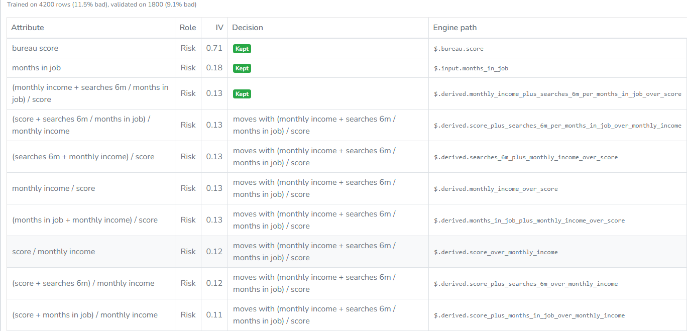
The first panel lists every risk attribute examined in the run, along with its role, its IV, the Decision taken about it, and the path where it is held.
IV, or information value, is a single measure of how well an attribute separates the outcome across all its bins. A higher value indicates a stronger separation, but IV is a ranking device rather than a verdict: an IV of 0.6 for an attribute that is effectively the answer in disguise is a warning, not a success.
The Decision column says Kept or gives the reason the attribute was not retained. The most common reason is "moves with credit score", meaning that the attribute carries much of the same information as an attribute already kept, so retaining both would count the same evidence twice. Attributes below the support floor, along with attributes whose bins show no separation, are also dropped at this point.
Suppressed attributes appear beneath the table with their role. They were never candidates; see Attribute roles.
Derived quantities tried
Analysts compute ratios before mining, and the pipeline does the same. Derived quantities tried lists what it built from your numeric attributes, including commitments over income, amount over income, amount over term, and similar measures. A derived quantity that earns its place appears in the binning and scorecard like any other characteristic, with a readable name and its path beside it.
This is often where the policy's real driver appears, because an affordability rule may depend on a ratio of three inputs that no single-attribute analysis can find.
Binning and stability
Each kept attribute is divided into fine bins first, then merged until the pattern is monotone and every bin meets the support floor. Sentinel values, such as -9 or -8 when they mean "no record" rather than a quantity, remain in their own bins instead of being averaged into a range where they do not belong. Categorical levels that are too thin to stand alone are folded into an "other" bin.
The table shows each attribute's role, IV, and bins in order. Show stability opens that attribute's time panel.
Three checks, and the worst one wins
Stability is assessed in three ways because each check catches a different failure.
| Check | Question it asks | What it misses |
|---|---|---|
| Population (PSI) | Has the mix moved between the periods, so that bins hold different shares of the book than they used to? | A stable mix whose bins behave differently |
| Order | Do the bins keep their ranking over time, so that the risky bin stays the risky one? | Bins in the right order that drift together |
| Rate swing | Does each bin's own bad rate hold between periods, once sampling noise is allowed for? | Nothing, but on a thin book it can only report "too few events" |
The panel reports the worst of the three conclusions and makes the disagreement explicit: "PSI alone would call this stable, but it is not." That prevents a single green number from concealing a problem.
Reading the stability panel
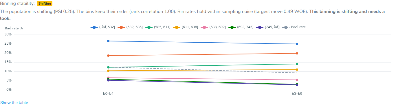
The panel begins with the population and order verdicts, each written as a sentence: "The population is shifting (PSI 0.14)", "The bins keep their order (rank correlation 0.95)", or "The bin order breaks down over time (rank correlation 0.41)".
Below them, a chart shows each bin's bad rate by period against the Pool rate, followed by a table with one row per bin:
| Column | What it says |
|---|---|
| Bin | The band |
| Rate swing | The largest move in this bin's evidence between periods, or Too few events when the bin has too few bad cases in a period to say anything |
| Calendar check | Whether the bin's effect survives being measured within each period. Not calendar-driven means it does |
The calendar check separates a real effect from one that belongs only to a particular period. If an attribute appears predictive because a bad campaign ran in March and that segment is unusually full of March cases, the effect disappears when each period is judged on its own, and the panel reports that rather than treating the finding as reliable.
When bins cross over time, the panel identifies them as merge candidates, since two bins that exchange positions between periods are not behaving as two distinct bins.
The final line gives the conclusion: "This binning is stable", "This binning is shifting and needs a look", "This binning is not stable", or "Stability cannot be judged yet" when the available window contains too little history to divide into periods.
Scorecard bins with WOE
The table shows the same bins with their weight of evidence and the points assigned by the fit, followed by a line describing the data used to build it: "Fitted on 5,890 rows. AUC train 0.81, validate 0.77." Weight of evidence is the logarithm of how the bad and good cases are distributed between a bin and the pool. A negative value means worse than average, a positive value means better, and zero means the bin adds no information.
Read this table alongside the points table to check that the scorecard is monotone in the direction your business expects. A bin that scores against the trend deserves investigation even when the numbers appear to support it.
Cutoff sheet
The cutoff sheet contains the sweep behind the curve, with one row for each score threshold and columns for the Approval rate, the Bad rate approved, and the Bad rate declined. It is calculated on the validation side only, using labeled rows, and its header gives the pool's base rate so every row has a reference point.
Read it in both directions: move down the approval column to find the volume you must hold, then across to the bad rate to see what that volume costs.
Cutoff by segment
Where product or channel attributes are available, the same sweep is repeated for each segment, showing at every global cutoff the approval rate within the segment and the bad rate among its approvals. The hint on the table states the calculation plainly: "Each cell: approval rate in the segment / bad rate among what it approves, at that global cutoff."
This shows whether a single cutoff is defensible or is really three cutoffs presented as one.
Overriding the binning
Two overrides sit above the binning table.
Drop selected and refit removes the variables you ticked and rebuilds everything downstream. Use it when an attribute is statistically strong but practically unusable because it is unavailable at decision time, about to be discontinued, or something you are not willing to decide on.
Ask AI to review sends the binning for a second opinion on its boundaries, typically returning proposed rounder cuts and merges that fit the way the business describes the attribute. The proposal is shown for you to approve with Apply and refit or dismiss; it only moves boundaries you can see, never invents a number, and cannot apply itself.
Either override requeues the pipeline, which answers "Pipeline requeued, recomputing on your version" and rebuilds the scorecard, cutoff, and record from your version. What you changed, together with the fact that you changed it, becomes part of the record.